This week, on a whim, I helped another lab with some analysis work and learned a bit about algorithms in the process. It turned out that the original Perl program ran quite slowly, so I thought about rewriting it in Python and then optimizing it further.
Algorithm Principle
In techniques like DamID-seq or ChIP-seq, since they essentially record a form of “affinity,” the data contains a lot of nonspecific affinity noise. Therefore, we need an algorithm to find specifically affinity peaks, avoiding mistaking noise generated by chance for specific affinity peaks.
The implementation idea of the find_peaks algorithm is actually quite simple, roughly divided into the following steps:
- Load data: The damidseq_pipeline aligns raw sequencing results to a reference genome and subsequently generates a
scorereflecting affinity. Each record also includes information likechr,start,end, corresponding to the genome, alignment start, and end positions. - Calculate percentiles: Sort the non-empty
scorevalues from the results, then calculate thescorevalue corresponding to specified percentiles (determined by the starting percentilemin_quantand step sizestep). - Calculate occurrence probability: Shuffle the records, then filter based on the percentile thresholds from step 2. If
min_countor more consecutive records meet the threshold, it’s considered a peak. RepeatNtimes, cumulatively recording the size and count of peaks found for each threshold. - Linear regression: For such calculations on randomly shuffled data, we can assume that values exceeding the threshold are uniformly distributed across the entire dataset. Therefore, the probability of encountering another qualifying value after one is constant. If the average number of observed peaks of length is , then we should have , where is a constant reflecting the density of values above the threshold. Thus, the relationship between observed peak count and size should follow an exponential distribution. Taking the logarithm of the observed counts allows us to fit a linear relationship.
- Count real occurrence frequency: Similar to step 3, but here we do not shuffle the records. We respect their chromosome assignment and sequential order, counting the relationship between peak size and number for each threshold.
- Calculate False Discovery Rate (FDR): The fitted relationship from step 4 gives one per percentile threshold. Using this result, we can predict the number of peaks of a specific size expected from purely random distribution for each threshold. Comparing this with the real observed number yields the FDR for observing a peak of that length at that threshold. By controlling the
FDR, we can determine the minimum length required for a peak to be considered significant under each threshold condition. - Identify significant peaks: Filter out the significant peaks based on the results from the previous step.
- Merge significant peaks: Merge significant peaks within the same chromosome (often duplicates from being significant under different thresholds), obtaining the maximum
scoreand minimumFDRfor overlapping peaks, and write the results to a file.
Replicating the Algorithm
With the above logic, writing the program was quick. To allow the program to run with minimal dependencies, we implemented all functionality using only Python’s built-in libraries. After writing this version, I tested the efficiency of the Perl and Python programs with a small N, with results roughly as follows:
| Perl | Python | |
|---|---|---|
| Time (sec) | 240s | ~210s |
Optimizing the Algorithm
Since the improvement wasn’t significant, we were certainly not satisfied. Running a profile with the amazing scalene revealed that a lot of time was spent checking if score was . This logic was originally copied from the Perl implementation, so for every record, whether calculating percentile thresholds or counting occurrence frequencies, it first needed to check if its score was and ignore it if so.
Thus, I tried using Python’s built-in filter function to filter the results, avoiding the if branch check (built-in implementations are generally faster):
def call_peaks_unified_redux(...): ... total = len(probes) for i in range(total): chrom, start, end, score = probes[i] if not score: continue for chrom, start, end, score in filter(lambda x: x[3], probes): ...Testing again showed good results, with a noticeable speed increase.
| Perl | Python | |
|---|---|---|
| Time (sec) | 240s | ~90s |
But! I was still not satisfied. This still took over a minute to run, and that was with a reduced iteration count. In practice, a larger N ensures that random sampling covers more possibilities, making the linear fit more accurate. So, we could think about further optimization.
Analyzing the code carefully, we can see:
load_gff: When loading the file, records withscoreof0orNAare also stored in the result array.find_quant: When encountering a record withscore0, it skips it, which doesn’t affect the result.find_randomised_peaks: When randomly shuffling records, if only a subset is specified, it might include records withscore0.call_peaks_unified_redux: When encountering a record withscore0, it skips it, which doesn’t affect the result.
Therefore, a large portion of the loaded data consists of records with score 0, but we don’t need to consider them in our calculations. Their only impact is in find_randomised_peaks when taking a subset. So, if we can handle this part of the logic properly, we can filter out these records upon loading, reducing subsequent computation.
First, rewrite the load_gff function to ignore empty records directly. To keep calculated metrics like coverage consistent, we move some logic from later functions here:
def load_gff(fn: str) -> list[PROBE]: global args, RAW_READS_NUM line_num = 0 total_coverage = 0 parsed_result: list[PROBE] = list() sys.stderr.write(f"Reading input file: {fn} ...\n") with open(fn, "r") as f: for line in f:14 collapsed lines
line_num += 1 if line_num % 10000 == 0: sys.stderr.write(f"Read {line_num} lines\r") ll = line.strip().split("\t") # skip empty lines if len(ll) < 4: continue if len(ll) == 4: # bedgraph chrom, start, end, score = ll else: # GFF chrom = ll[0] start, end, score = ll[3:6] # increment raw reads number RAW_READS_NUM += 1 # skip empty reads if not args.no_discard_zeros and (score == "NA" or not float(score)): continue # record read parsed_result.append( ( CHROM(chrom), START(POS(int(start))), END(POS(int(end))), SCORE(float(score) if score != "NA" else 0), ) ) # record total coverage total_coverage += int(end) - int(start) sys.stderr.write(f"Read {line_num} lines\n") sys.stderr.write("Sorting ...\n") parsed_result = sorted(parsed_result, key=lambda x: (x[0], x[1])) sys.stderr.write(f"Total coverage was {total_coverage} bp\n") return parsed_resultThen, in the find_quant function, no extra checks are needed:
def find_quant(probes: list[PROBE]): global args total_coverage = 0 frags: list[SCORE] = list() for (chrom, start, end, score) in filter(lambda x: x[3], probes): total_coverage += end - start frags.append(score) frags = [x[3] for x in probes] frags = sorted(frags) sys.stderr.write(f"Total coverage was {total_coverage} bp\n")8 collapsed lines
quants = [ (q * args.step, int(q * args.step * len(frags)) - 1) for q in range(math.ceil(args.min_quant / args.step), math.ceil(1 / args.step)) ] for cut_off, score_idx in quants: sys.stdout.write(f"\tQuantile {cut_off:0.2f}: {frags[score_idx]:0.2f}\n") peakmins = [THRESH(frags[score_idx]) for (_, score_idx) in quants] return peakminsThe same applies to call_peaks_unified_redux:
def call_peaks_unified_redux(...): ... for pm in peakmins: ... for chrom, start, end, score in filter(lambda x: x[3], probes): for chrom, start, end, score in probes: ...find_randomised_peaks is a bit more complex, but we can still do no worse than the original. In the original program, if frac was specified, only the fixed first frac records (where frac is an integer) were used to estimate expected frequency. This meant the proportion of empty records in the first frac could be greater or less than their overall proportion, and this bias would appear in every shuffle. So, we adopt a more general approach:
- Let
fracbe a float , representing the proportion of records we need. - When generating the dataset, simulate taking records from the total , and calculate the number of non-empty records within that sample.
- Use as the sample size to sample from the non-empty records. The resulting subset is used for expectation estimation.
def find_randomised_peaks(probes: list[PROBE], peakmins: list[THRESH]):5 collapsed lines
global args, RAW_READS_NUM peak_count = None sys.stdout.write("Duplicating ...\n") pbs = probes.copy() sys.stdout.write("Calling peaks on input file ...\n") for iter_num in range(args.n): sys.stdout.write(f"Iteration {iter_num+1}: [shuffling ...] \r") # This is a naive approximation to randomly sample a fraction # as the full sequence doesn't contain empty reads # (but no worse than the original approach anyway) if args.frac: pbs = pbs[: args.frac] num_to_sample = sum( map( # This makes sure that it works for both # data including and excluding empty reads lambda x: x <= int(len(probes) * args.frac), random.sample(range(RAW_READS_NUM), int(RAW_READS_NUM * args.frac)), ) )7 collapsed lines
pbs = random.sample(probes, num_to_sample) # The built-in shuffle uses the same algorithm (Fisher-Yates) # as the original Perl program random.shuffle(pbs) _, peak_count = call_peaks_unified_redux( iter_num, pbs, peakmins, None, peak_count ) return peak_countOther minor adjustments were made to align with these changes, but they are straightforward and won’t be listed one by one.
We tested again, and the results were amazing!
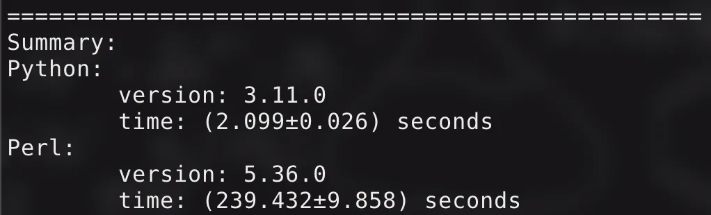
Running with default parameters (N: , fdr: , min_count: , min_quant: , step: ), the original Perl program took about minutes, while the current Python program only needs about ten seconds. The intuitive feeling is:
 The improvement is very perceptible! The code has been open-sourced under the GPLv3 license, repository link.